Visualizing TCP
Posted on Monday, December 13, 2010.
This video depicts an HTTP GET by showing packets as balls flying between client and server, slowed 40x compared to real time. It's pretty nice for getting a visceral sense of the underlying TCP session: you can see individual rounds at the start and then as the session stabilizes the rounds begin to overlap enough that they disappear.
When I saw the video, it reminded me of the ever-present videos of sorting algorithms, like the ones on the Wikipedia heapsort and quicksort pages:

That in turn reminded me of a 2007 blog post by Aldo Cortesi about visualizing sorting algorithms using graphs instead of videos. He points out that the animations make time-based questions difficult to answer:
[It] is my measured opinion that this animation has all the explanatory power of a glob of porridge flung against a wall. To see why I say this, try to find rough answers to the following set of simple questions with reference to it:
- After what percentage of time is half of the array sorted?
- Can you find an element that moved about half the length of the array to reach its final destination?
- What percentage of the array was sorted after 80% of the sorting process? How about 20%?
- Does the number of sorted elements grow linearly or non-linearly with time (i.e. logarithmically or exponentially)?
If you thought that was harder than it needed to be, blame animation. First, while humans are great at estimating distances in space, they are pretty bad at estimating distances in time. This is why you had to watch the animation two or three times to answer the first question. When we translate time to a geometric length, as is done in any scientific diagram with a time dimension, this estimation process becomes easy. Second, many questions about sorting algorithms require us to actively compare the sorting state at two or more different time points. Since we don't have perfect memories, this is very, very hard in all but the simplest cases. This leaves us with a strangely one-dimensional view into an animation - we can see what's on screen at any given moment, but we have to strain to answer simple questions about, say, rates of change. Which is why the final question is hard to answer accurately.
Instead, he suggests plotting static graphs showing the paths of individual array elements over time. Here are his original visualizations of heapsort and quicksort:
The blog post is worth reading in full. It has much more detail and links to many other interesting blog posts and a new site dedicated to those visualizations, sortvis.org.
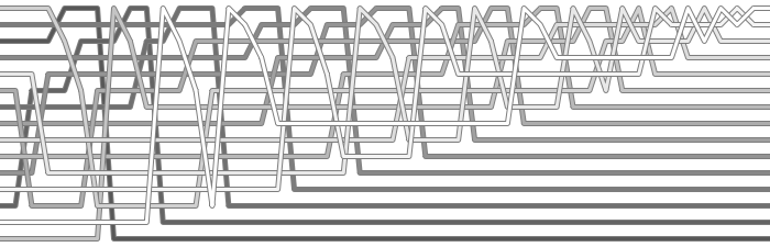
Remembering this made me wonder if the lesson of the sorting animations applied to the TCP animations too, so I collected my own tcpdumps of both sides of an HTTP GET, pulled out the trusty (but neglected) Unix tool join(1) to produce a dump with two timestamps on each packet, and then used Perl to turn it into a graph (raw PostScript):
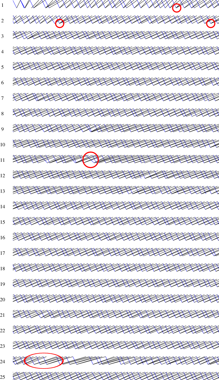
Time marches to the right, with each row picking up where the previous one left off. Blue lines indicate packets from the client and black lines indicate packets from the server.
I think this kind of graph has the same important benefits that Cortesi realized with his sorting graphs. It's static, so you have time to study it, focus on anomalies, or notice patterns that aren't immediately apparent. The geometry of the lines, with flatter slopes corresponding to slower packets, makes it easy to compare speeds.
Here are just a few things I noticed.
The connection starts with the usual 3-way TCP handshake. The client sends the third packet in the handshake and the first data packet back to back, one of its few back-to-back transmissions. After the handshake and the initial GET, which probably fits entirely in that first packet, the client only receives data: the black lines are large payloads while the blue lines are ACK messages that trigger more payloads. Scanning across the client's view of the connection (the top edge of each row) we can see that the client is using the standard delayed ACKs, sending an ACK every two packets. Scanning across the server's view of the connection (the bottom edge of each row) we can see that the server usually responds to the acknowledgement of two packets by sending two more packets, leaving the TCP window size (the number of packets in flight) unchanged. Occasionally, though, the server grows the window size by responding with three packets instead of two. Three of these events are circled in rows 1 and 2. Occasionally the server only responds to an ACK with a single packet, but most of those appear to be times when the client was only acknowledging a single packet.
We can count the number of packets in flight at any given time by counting the number of black lines that cross a particular blue line, plus the number of packets sent when the blue line reaches the server. For example, three black lines cross the last complete blue line on row 1, and the server sends two more packets in response, so the window size then is five packets. By the end of row 2, the window size is seven packets.
The window size fluctuates a little once it stabilizes: at the end of row 10 it has grown to eight packets but at the end of row 20 it is back to seven. It's not clear what causes the server to shrink or grow the window size. I couldn't find any evidence of packet loss in the traces.
I set the time axis such that those initial packets travel on lines with a 2:1 slope. A glance down the page shows that while the packets sent by the client continue to travel at approximately that speed, the packets sent by the server gradually slow until row 3, where they appear to stabilize around a 1:2 slope, four times longer to send than the initial packets. Looking at the raw data, those later packets around 100 ms for a one-way trip compared to 20 ms during the original handshake, so our visual estimate is not far off. This is evidence of queueing along the path from server to client; the likely suspect is the server's upstream DSL connection.
The circled fragment on row 11 is more evidence of queuing. Something delays the ACK from client to server (note the more gradual slope) but the packets that the server sends in response are not noticeably delayed: they still had time to catch up with the bottlenecked packets.
The circled fragment on row 24 shows the opposite case. Most of the time the packet arrivals at the client are evenly spaced, but if a few packets from the server to the client get delayed, that delays the corresponding ACKs, which throws the conversation into a bursty behavior that takes a few rounds to convert to a steady state.
People more familiar with TCP might notice other interesting details in the plot. If you find something, please leave a comment.
Of course, the idea of plotting network packets against time in this way is not new: any class in network protocols uses diagrams like these. However, I have never seen a diagram like this one made from real timings on both sides, so that you can see the actual speeds of individual packets and compare the relative speeds of different packets, and I've never seen a diagram that was this zoomed out, so that you can see macro effects like the occasional congestion burp of rows 11 and 24. It would be interesting to have a tool that generated these automatically, but I rarely have a need to examine protocols at this level so I'm not likely to spend more time on it. If you know of (or make) such a tool, please leave a comment.
(Comments originally posted via Blogger.)
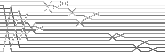
Soapbox Cicero (December 13, 2010 12:19 PM) Fascinating post as usual, Russ. But I found the chart a little hard to read, personally. I opened it up in gimp and switched the blue and red and found it much easier to follow:
http://i.imgur.com/pCeyM.png
Anonymous (December 13, 2010 3:46 PM) OPNET's ITGuru ACE product creates beautiful plots of packet's transmission/flight/reception times.
They are used extensively in debugging networked application performance. I hadn't realized that the feature was uncommon.
Bizarrely, I can't find any screenshots online.
http://opnet.com is the main company site.
Anonymous (December 13, 2010 3:50 PM) I found an example of the packet-transmission screenshots I mentioned in my previous comment:
See Page 6-5 (and others) of this PDF:
https://www.cisco.com/en/US/docs/net_mgmt/application_analysis_solution/1.0/tutorials_and_examples/tut_ace.pdf
Jim (January 7, 2011 3:46 PM) Interesting. Switching the colours helped; but with such a long transaction the very long X axis makes some comparisons difficult.
I liked the interpretation of the window size; but for actual traffic analysis I think it would be useful to have data like that explicitly labelled on the graph, along with highlights for important packet types (SYN, FIN, and so on). Hopefully there are not so many of these that they swamp the labelling. Otherwise much of the useful interpretation of this graph is down to manually counting lines.
Another possibility is charting the second order for window size, and showing the rate of change of window size over time (i.e. acceleration instead of velocity); that way we could see when changes from the ideal behaviour happen.
Grabbing an explicit visualisation of the packet trip time/speed would also be interesting, as this impacts on the window size.