The Magic of Sampling, and its Limitations

Posted on Saturday, February 4, 2023.

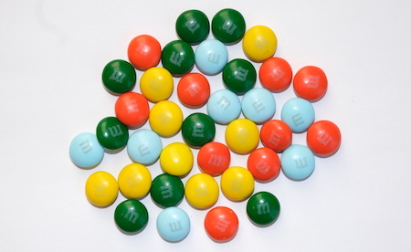
Suppose I have a large number of M&Ms and want to estimate what fraction of them have Peter’s face on them. As one does.

If I am too lazy to count them all, I can estimate the true fraction using sampling: pick N at random, count how many P have Peter’s face, and then estimate the fraction to be P/N.

I can write a Go program to pick 10 of the 37 M&Ms for me: 27 30 1 13 36 5 33 7 10 19. (Yes, I am too lazy to count them, but I was not too lazy to number the M&Ms in order to use the Go program.)

Based on this estimate, we can estimate that 3/10 = 30% of my M&Ms have Peter’s face. We can do it a few more times:

And we get a few new estimates: 30%, 40%, 20%. The actual fraction turns out to be 9/37 = 24.3%. These estimates are perhaps not that impressive, but we are only using 10 samples. With not too many more samples, we can get far more accurate estimates, even for much larger data sets. Suppose we had many more M&Ms, again 24.3% Peter faces, and we sample 100 of them, or 1,000, or 10,000. Since we’re lazy, let’s write a program to simulate the process.

$ go run sample.go
   10: 40.0% 20.0% 30.0%  0.0% 10.0% 30.0% 10.0% 20.0% 20.0%  0.0%
  100: 25.0% 26.0% 21.0% 26.0% 15.0% 25.0% 30.0% 30.0% 29.0% 20.0%
 1000: 24.7% 23.8% 21.0% 25.4% 25.1% 24.2% 25.7% 22.9% 24.0% 23.8%
10000: 23.4% 24.6% 24.3% 24.3% 24.7% 24.6% 24.6% 24.7% 24.1% 25.0%
$

Accuracy improves fairly quickly:

• With 10 samples, our estimates are accurate to within about 15%.
• With 100 samples, our estimates are accurate to within about 5%.
• With 1,000 samples, our estimates are accurate to within about 3%.
• With 10,000 samples, our estimates are accurate to within about 1%.

Because we are estimating only the percentage of Peter faces, not the total number, the accuracy (also measured in percentages) does not depend on the total number of M&Ms, only on the number of samples. So 10,000 samples is enough to get roughly 1% accuracy whether we have 100,000 M&Ms, 1 million M&Ms, or even 100 billion M&Ms! In the last scenario, we have 1% accuracy despite only sampling 0.00001% of the M&Ms.

The magic of sampling is that we can derive accurate estimates about a very large population using a relatively small number of samples.

Sampling turns many one-off estimations into jobs that are feasible to do by hand. For example, suppose we are considering revising an error-prone API and want to estimate how often that API is used incorrectly. If we have a way to randomly sample uses of the API (maybe grep -Rn pkg.Func . | shuffle -m 100), then manually checking 100 of them will give us an estimate that’s accurate to within 5% or so. And checking 1,000 of them, which may not take more than an hour or so if they’re easy to eyeball, improves the accuracy to 1.5% or so. Real data to decide an important question is usually well worth a small amount of manual effort.

For the kinds of decisions I look at related to Go, this approach comes up all the time: What fraction of for loops in real code have a loop scoping bug? What fraction of warnings by a new go vet check are false positives? What fraction of modules have no dependencies? These are drawn from my experience, and so they may seem specific to Go or to language development, but once you realize that sampling makes accurate estimates so easy to come by, all kind of uses present themselves. Any time you have a large data set,

select * from data order by random() limit 1000;

is a very effective way to get a data set you can analyze by hand and still derive many useful conclusions from.

Accuracy

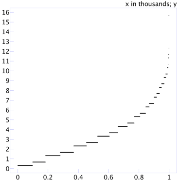
Let’s work out what accuracy we should expect from these estimates. The brute force approach would be to run many samples of a given size and calculate the accuracy for each. This program runs 1,000 trials of 100 samples each, calculating the observed error for each estimate and then printing them all in sorted order. If we plot those points one after the other along the x axis, we get a picture like this:

The data viewer I’m using in this screenshot has scaled the x-axis labels by a factor of 1,000 (“x in thousands”). Eyeballing the scatterplot, we can see that half the time the error is under 3%, and 80% of the time the error is under 5½%.

We might wonder at this point whether the error depends on the actual answer (24.3% in our programs so far). It does: the error will be lower when the population is lopsided. Obviously, if the M&Ms are 0% or 100% Peter faces, our estimates will have no error at all. In a slightly less degenerate case, if the M&Ms are 1% or 99% Peter faces, the most likely estimate from just a few samples is 0% or 100%, which has only 1% error. It turns out that, in general, the error is maximized when the actual fraction is 50%, so we’ll use that for the rest of the analysis.

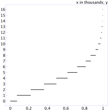
With an actual fraction of 50%, 1,000 sorted errors from estimating by sampling 100 values look like:

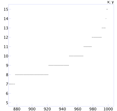
The errors are a bit larger. Now the half the time the error is 4% and 80% of the time the error is 6%. Zooming in on the tail end of the plot produces:

We can see that 90% of the trials have error 8% or less, 95% of the trials have error 10% or less, and 99% of the trials have error 12% or less. The statistical way to phrase those statements is that “a sample of size N = 100 produces a margin of error of 8% with 90% confidence, 10% with 95% confidence, and 12% with 99% confidence.”

Instead of eyeballing the graphs, we can update the program to compute these numbers directly.

$ go run sample.go
N =    10: 90%: 30.00% 95%: 30.00% 99%: 40.00%
N =   100: 90%:  9.00% 95%: 11.00% 99%: 13.00%
N =  1000: 90%:  2.70% 95%:  3.20% 99%:  4.30%
N = 10000: 90%:  0.82% 95%:  0.98% 99%:  1.24%
$

There is something meta about using sampling (of trials) to estimate the errors introduced by sampling of an actual distribution. What about the error being introduced by sampling the errors? We could instead write a program to count all possible outcomes and calculate the exact error distribution, but counting won’t work for larger sample sizes. Luckily, others have done the math for us and even implemented the relevant functions in Go’s standard math package. The margin of error for a given confidence level and sample size is:

func moe(confidence float64, N int) float64 {
    return math.Erfinv(confidence) / math.Sqrt(2 * float64(N))
}

That lets us compute the table more directly.

$ go run sample.go
N =     10: 90%: 26.01% 95%: 30.99% 99%: 40.73%
N =     20: 90%: 18.39% 95%: 21.91% 99%: 28.80%
N =     50: 90%: 11.63% 95%: 13.86% 99%: 18.21%
N =    100: 90%:  8.22% 95%:  9.80% 99%: 12.88%
N =    200: 90%:  5.82% 95%:  6.93% 99%:  9.11%
N =    500: 90%:  3.68% 95%:  4.38% 99%:  5.76%
N =   1000: 90%:  2.60% 95%:  3.10% 99%:  4.07%
N =   2000: 90%:  1.84% 95%:  2.19% 99%:  2.88%
N =   5000: 90%:  1.16% 95%:  1.39% 99%:  1.82%
N =  10000: 90%:  0.82% 95%:  0.98% 99%:  1.29%
N =  20000: 90%:  0.58% 95%:  0.69% 99%:  0.91%
N =  50000: 90%:  0.37% 95%:  0.44% 99%:  0.58%
N = 100000: 90%:  0.26% 95%:  0.31% 99%:  0.41%
$

We can also reverse the equation to compute the necessary sample size from a given confidence level and margin of error:

func N(confidence, moe float64) int {
    return int(math.Ceil(0.5 * math.Pow(math.Erfinv(confidence)/moe, 2)))
}

That lets us compute this table.

$ go run sample.go
moe = 5%:  90%:   271  95%:   385  99%:   664
moe = 2%:  90%:  1691  95%:  2401  99%:  4147
moe = 1%:  90%:  6764  95%:  9604  99%: 16588
$

To accurately estimate the fraction of items with a given property, like M&Ms with Peter faces, each item must have the same chance of being selected, as each M&M did. Suppose instead that we had ten bags of M&Ms: nine one-pound bags with 500 M&Ms each, and a small bag containing the 37 M&Ms we used before. If we want to estimate the fraction of M&Ms with Peter faces, it would not work to sample by first picking a bag at random and then picking an M&M at random from the bag. The chance of picking any specific M&M from a one-pound bag would be 1/10 × 1/500 = 1/5,000, while the chance of picking any specific M&M from the small bag would be 1/10 × 1/37 = 1/370. We would end up with an estimate of around 9/370 = 2.4% Peter faces, even though the actual answer is 9/(9×500+37) = 0.2% Peter faces.

The problem here is not the kind of random sampling error that we computed in the previous section. Instead it is a systematic error caused by a sampling mechanism that does not align with the statistic being estimated. We could recover an accurate estimate by weighting an M&M found in the small bag as only w = 37/500 of an M&M in both the numerator and denominator of any estimate. For example, if we picked 100 M&Ms with replacement from each bag and found 24 Peter faces in the small bag, then instead of 24/1000 = 2.4% we would compute 24w/(900+100w) = 0.2%.

As a less contrived example, Go’s memory profiler aims to sample approximately one allocation per half-megabyte allocated and then derive statistics about where programs allocate memory. Roughly speaking, to do this the profiler maintains a sampling trigger, initialized to a random number between 0 and one million. Each time a new object is allocated, the profiler decrements the trigger by the size of the object. When an allocation decrements the trigger below zero, the profiler samples that allocation and then resets the trigger to a new random number between 0 and one million.

This byte-based sampling means that to estimate the fraction of bytes allocated in a given function, the profiler can divide the total sampled bytes allocated in that function divided by the total sampled bytes allocated in the entire program. Using the same approach to estimate the fraction of objects allocated in a given function would be inaccurate: it would overcount large objects and undercount small ones, because large objects are more likely to be sampled. In order to recover accurate statistics about allocation counts, the profiler applies a size-based weighting function during the calcuation, just as in the M&M example. (This is the reverse of the situation with the M&Ms: we are randomly sampling individual bytes of allocated memory but now want statistics about their “bags”.)

It is not always possible to undo skewed sampling, and the skew makes margin of error calculation more difficult too. It is almost always better to make sure that the sampling is aligned with the statistic you want to compute.