Transparent Logs for Skeptical Clients
Posted on Friday, March 1, 2019.
PDF
Suppose we want to maintain and publish a public, append-only log of data. Suppose also that clients are skeptical about our correct implementation and operation of the log: it might be to our advantage to leave things out of the log, or to enter something in the log today and then remove it tomorrow. How can we convince the client we are behaving?
This post is about an elegant data structure we can use to publish a log of N records with these three properties:
- For any specific record R in a log of length N, we can construct a proof of length O(lg N) allowing the client to verify that R is in the log.
- For any earlier log observed and remembered by the client, we can construct a proof of length O(lg N) allowing the client to verify that the earlier log is a prefix of the current log.
- An auditor can efficiently iterate over the records in the log.
(In this post, “lg N” denotes the base-2 logarithm of N, reserving the word “log” to mean only “a sequence of records.”)
The Certificate Transparency project publishes TLS certificates in this kind of log. Google Chrome uses property (1) to verify that an enhanced validation certificate is recorded in a known log before accepting the certificate. Property (2) ensures that an accepted certificate cannot later disappear from the log undetected. Property (3) allows an auditor to scan the entire certificate log at any later time to detect misissued or stolen certificates. All this happens without blindly trusting that the log itself is operating correctly. Instead, the clients of the log—Chrome and any auditors—verify correct operation of the log as part of accessing it.
This post explains the design and implementation
of this verifiably tamper-evident log,
also called a transparent log.
To start, we need some cryptographic building blocks.
Cryptographic Hashes, Authentication, and Commitments
A cryptographic hash function is a deterministic function H that maps an arbitrary-size message M to a small fixed-size output H(M), with the property that it is infeasible in practice to produce any pair of distinct messages M1 ≠ M2 with identical hashes H(M1) = H(M2). Of course, what is feasible in practice changes. In 1995, SHA-1 was a reasonable cryptographic hash function. In 2017, SHA-1 became a broken cryptographic hash function, when researchers identified and demonstrated a practical way to generate colliding messages. Today, SHA-256 is believed to be a reasonable cryptographic hash function. Eventually it too will be broken.
A (non-broken) cryptographic hash function provides a way to bootstrap a small amount of trusted data into a much larger amount of data. Suppose I want to share a very large file with you, but I am concerned that the data may not arrive intact, whether due to random corruption or a man-in-the-middle attack. I can meet you in person and hand you, written on a piece of paper, the SHA-256 hash of the file. Then, no matter what unreliable path the bits take, you can check whether you got the right ones by recomputing the SHA-256 hash of the download. If it matches, then you can be certain, assuming SHA-256 has not been broken, that you downloaded the exact bits I intended. The SHA-256 hash authenticates—that is, it proves the authenticity of—the downloaded bits, even though it is only 256 bits and the download is far larger.
We can also turn the scenario around, so that, instead of distrusting the network, you distrust me. If I tell you the SHA-256 of a file I promise to send, the SHA-256 serves as a verifiable commitment to a particular sequence of bits. I cannot later send a different bit sequence and convince you it is the file I promised.
A single hash can be an authentication or commitment
of an arbitrarily large amount of data,
but verification then requires hashing the entire data set.
To allow selective verification of subsets of the data,
we can use not just a single hash
but instead a balanced binary tree of hashes,
known as a Merkle tree.
Merkle Trees
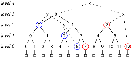
A Merkle tree is constructed from N records, where N is a power of two. First, each record is hashed independently, producing N hashes. Then pairs of hashes are themselves hashed, producing N/2 new hashes. Then pairs of those hashes are hashed, to produce N/4 hashes, and so on, until a single hash remains. This diagram shows the Merkle tree of size N = 16:
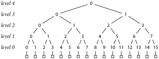
The boxes across the bottom represent the 16 records. Each number in the tree denotes a single hash, with inputs connected by downward lines. We can refer to any hash by its coordinates: level L hash number K, which we will abbreviate h(L, K). At level 0, each hash’s input is a single record; at higher levels, each hash’s input is a pair of hashes from the level below.
h(0, K) = H(record K)
h(L+1, K) = H(h(L, 2 K), h(L, 2 K+1))
To prove that a particular record is contained in the tree represented by a given top-level hash (that is, to allow the client to authenticate a record, or verify a prior commitment, or both), it suffices to provide the hashes needed to recompute the overall top-level hash from the record’s hash. For example, suppose we want to prove that a certain bit string B is in fact record 9 in a tree of 16 records with top-level hash T. We can provide those bits along with the other hash inputs needed to reconstruct the overall tree hash using those bits. Specifically, the client can derive as well as we can that:
T = h(4, 0)
= H(h(3, 0), h(3, 1))
= H(h(3, 0), H(h(2, 2), h(2, 3)))
= H(h(3, 0), H(H(h(1, 4), h(1, 5)), h(2, 3)))
= H(h(3, 0), H(H(H(h(0, 8), h(0, 9)), h(1, 5)), h(2, 3)))
= H(h(3, 0), H(H(H(h(0, 8), H(record 9)), h(1, 5)), h(2, 3)))
= H(h(3, 0), H(H(H(h(0, 8), H(B)), h(1, 5)), h(2, 3)))
If we give the client the values [h(3, 0), h(0, 8), h(1, 5), h(2, 3)], the client can calculate H(B) and then combine all those hashes using the formula and check whether the result matches T. If so, the client can be cryptographically certain that B really is record 9 in the tree with top-level hash T. In effect, proving that B is a record in the Merkle tree with hash T is done by giving a verifiable computation of T with H(B) as an input.
Graphically, the proof consists of the sibling hashes (circled in blue) of nodes along the path (highlighted in yellow) from the record being proved up to the tree root.
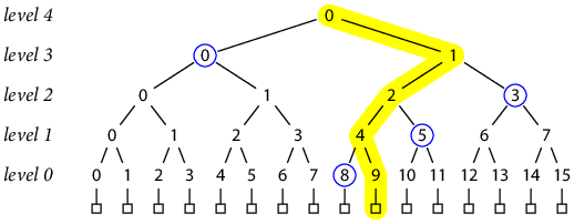
In general, the proof that a given record is contained in the tree requires lg N hashes, one for each level below the root.
Building our log as a sequence of records
hashed in a Merkle tree would give us a way to write
an efficient (lg N-length) proof that a particular record
is in the log.
But there are two related problems to solve:
our log needs to be defined for any length N,
not just powers of two,
and we need to be able to write
an efficient proof that one log is a prefix of another.
A Merkle Tree-Structured Log
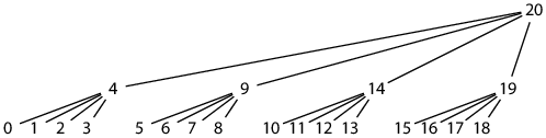
To generalize the Merkle tree to non-power-of-two sizes, we can write N as a sum of decreasing powers of two, then build complete Merkle trees of those sizes for successive sections of the input, and finally hash the at-most-lg N complete trees together to produce a single top-level hash. For example, 13 = 8 + 4 + 1:
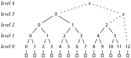
The new hashes marked “x” combine the complete trees, building up from right to left, to produce the overall tree hash. Note that these hashes necessarily combine trees of different sizes and therefore hashes from different levels; for example, h(3, x) = H(h(2, 2), h(0, 12)).
The proof strategy for complete Merkle trees applies equally well to these incomplete trees. For example, the proof that record 9 is in the tree of size 13 is [h(3, 0), h(0, 8), h(1, 5), h(0, 12)]:
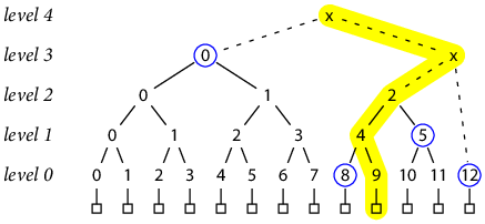
Note that h(0, 12) is included in the proof because it is the sibling of h(2, 2) in the computation of h(3, x).
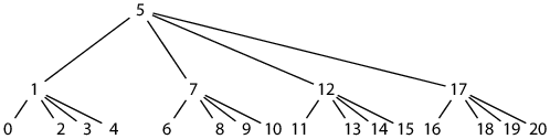
We still need to be able to write an efficient proof that the log of size N with tree hash T is a prefix of the log of size N′ (> N) with tree hash T′. Earlier, proving that B is a record in the Merkle tree with hash T was done by giving a verifiable computation of T using H(B) as an input. To prove that the log with tree hash T is included in the log with tree hash T′, we can follow the same idea: give verifiable computations of T and T′, in which all the inputs to the computation of T are also inputs to the computation of T′. For example, consider the trees of size 7 and 13:
In the diagram, the “x” nodes complete the tree of size 13 with hash T13, while the “y” nodes complete the tree of size 7 with hash T7. To prove that T7’s leaves are included in T13, we first give the computation of T7 in terms of complete subtrees (circled in blue):
T7 = H(h(2, 0), H(h(1, 2), h(0, 6)))
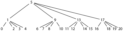
Then we give the computation of T13, expanding hashes as needed to expose the same subtrees. Doing so exposes sibling subtrees (circled in red):
T13 = H(h(3, 0), H(h(2, 2), h(0, 12)))
= H(H(h(2, 0), h(2, 1)), H(h(2, 2), h(0, 12)))
= H(H(h(2, 0), H(h(1, 2), h(1, 3))), H(h(2, 2), h(0, 12)))
= H(H(h(2, 0), H(h(1, 2), H(h(0, 6), h(0, 7)))), H(h(2, 2), h(0, 12)))
Assuming the client knows the trees have sizes 7 and 13, it can derive the required decomposition itself. We need only supply the hashes [h(2, 0), h(1, 2), h(0, 6), h(0, 7), h(2, 2), h(0, 12)]. The client recalculates the T7 and T13 implied by the hashes and checks that they match the originals.
Note that these proofs only use hashes for completed subtrees—that is, numbered hashes,
never the “x” or “y” hashes that combine differently-sized subtrees.
The numbered hashes are permanent,
in the sense that once such a hash appears in a
tree of a given size, that same hash will appear in all
trees of larger sizes.
In contrast, the “x” and “y” hashes are ephemeral—computed
for a single tree and never seen again.
The hashes common to the decomposition of two different-sized trees
therefore must always be permanent hashes.
The decomposition of the larger tree could make use of ephemeral
hashes for the exposed siblings,
but we can easily use only
permanent hashes instead.
In the example above,
the reconstruction of T13
from the parts of T7
uses h(2, 2) and h(0, 12)
instead of assuming access to T13’s h(3, x).
Avoiding the ephemeral hashes extends the maximum
record proof size from lg N hashes to 2 lg N hashes
and the maximum tree proof size from 2 lg N hashes
to 3 lg N hashes.
Note that most top-level hashes,
including T7 and T13,
are themselves ephemeral hashes,
requiring up to lg N permanent hashes to compute.
The exceptions are the power-of-two-sized trees
T1, T2, T4, T8, and so on.
Storing a Log
Storing the log requires only a few append-only files. The first file holds the log record data, concatenated. The second file is an index of the first, holding a sequence of int64 values giving the start offset of each record in the first file. This index allows efficient random access to any record by its record number. While we could recompute any hash tree from the record data alone, doing so would require N–1 hash operations for a tree of size N. Efficient generation of proofs therefore requires precomputing and storing the hash trees in some more accessible form.
As we noted in the previous section, there is significant commonality between trees. In particular, the latest hash tree includes all the permanent hashes from all earlier hash trees, so it is enough to store “only” the latest hash tree. A straightforward way to do this is to maintain lg N append-only files, each holding the sequence of hashes at one level of the tree. Because hashes are fixed size, any particular hash can be read efficiently by reading from the file at the appropriate offset.
To write a new log record, we must append the record data to the data file, append the offset of that data to the index file, and append the hash of the data to the level-0 hash file. Then, if we completed a pair of hashes in the level-0 hash file, we append the hash of the pair to the level-1 hash file; if that completed a pair of hashes in the level-1 hash file, we append the hash of that pair to the level-2 hash file; and so on up the tree. Each log record write will append a hash to at least one and at most lg N hash files, with an average of just under two new hashes per write. (A binary tree with N leaves has N–1 interior nodes.)
It is also possible to interlace lg N append-only hash files into a single append-only file, so that the log can be stored in only three files: record data, record index, and hashes. See Appendix A for details. Another possibility is to store the log in a pair of database tables, one for record data and one for hashes (the database can provide the record index itself).
Whether in files or in database tables, the stored form of the log is append-only, so cached data never goes stale, making it trivial to have parallel, read-only replicas of a log. In contrast, writing to the log is inherently centralized, requiring a dense sequence numbering of all records (and in many cases also duplicate suppression). An implementation using the two-table database representation can delegate both replication and coordination of writes to the underlying database, especially if the underlying database is globally-replicated and consistent, like Google Cloud Spanner or CockroachDB.
It is of course not enough just to store the log.
We must also make it available to clients.
Serving a Log
Remember that each client consuming the log is skeptical about the log’s correct operation. The log server must make it easy for the client to verify two things: first, that any particular record is in the log, and second, that the current log is an append-only extension of a previously-observed earlier log.
To be useful, the log server must also make it easy to find a record given some kind of lookup key, and it must allow an auditor to iterate over the entire log looking for entries that don’t belong.
To do all this, the log server must answer five queries:
-
Latest() returns the current log size and top-level hash, cryptographically signed by the server for non-repudiation.
-
RecordProof(R, N) returns the proof that record R is contained in the tree of size N.
-
TreeProof(N, N′) returns the proof that the tree of size N is a prefix of the tree of size N′.
-
Lookup(K) returns the record index R matching lookup key K, if any.
-
Data(R) returns the data associated with record R.
Verifying a Log
The client uses the first three queries to maintain a cached copy of the most recent log it has observed and make sure that the server never removes anything from an observed log. To do this, the client caches the most recently observed log size N and top-level hash T. Then, before accepting data bits B as record number R, the client verifies that R is included in that log. If necessary (that is, if R ≥ its cached N), the client updates its cached N, T to those of the latest log, but only after verifying that the latest log includes everything from the current cached log. In pseudocode:
validate(bits B as record R):
    if R ≥ cached.N:
        N, T = server.Latest()
        if server.TreeProof(cached.N, N) cannot be verified:
            fail loudly
        cached.N, cached.T = N, T
    if server.RecordProof(R, cached.N) cannot be verified using B:
        fail loudly
    accept B as record R
The client’s proof verification ensures that the log server is behaving correctly, at least as observed by the client. If a devious server can distinguish individual clients, it can still serve different logs to different clients, so that a victim client sees invalid entries never exposed to other clients or auditors. But if the server does lie to a victim, the fact that the victim requires any later log to include what it has seen before means the server must keep up the lie, forever serving an alternate log containing the lie. This makes eventual detection more likely. For example, if the victim ever arrived through a proxy or compared its cached log against another client, or if the server ever made a mistake about which clients to lie to, the inconsistency would be readily exposed. Requiring the server to sign the Latest() response makes it impossible for the server to disavow the inconsistency, except by claiming to have been compromised entirely.
The client-side checks are a little bit like how
a Git client maintains its own
cached copy of a remote repository and then,
before accepting an update during git pull,
verifies that the remote repository includes all local commits.
But the transparent log client only needs to
download lg N hashes for the verification,
while Git downloads all cached.N – N new data records,
and more generally, the transparent log client
can selectively read and authenticate individual
entries from the log,
without being required to download and store
a full copy of the entire log.
Tiling a Log
As described above, storing the log requires simple, append-only storage linear in the total log size, and serving or accessing the log requires network traffic only logarithmic in the total log size. This would be a completely reasonable place to stop (and is where Certificate Transparency as defined in RFC 6962 stops). However, one useful optimization can both cut the hash storage in half and make the network traffic more cache-friendly, with only a minor increase in implementation complexity. That optimization is based on splitting the hash tree into tiles, like Google Maps splits the globe into tiles.
A binary tree can be split into tiles of fixed height H and width 2H. For example, here is the permanent hash tree for the log with 27 records, split into tiles of height 2:
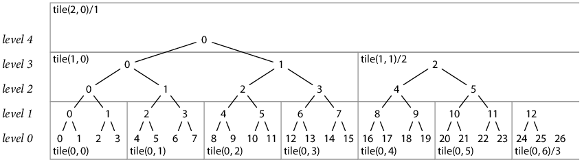
We can assign each tile a two-dimensional coordinate, analogous to the hash coordinates we’ve been using:
tile(L, K) denotes the tile at tile level L
(hash levels H·L up to H·(L+1)), Kth from the left.
For any given log size, the rightmost tile at each level
may not yet be complete:
the bottom row of hashes may contain only W < 2H hashes.
In that case we will write tile(L, K)/W.
(When the tile is complete, the “/W” is omitted, understood to be 2H.)
Storing Tiles
Only the bottom row of each tile needs to be stored: the upper rows can be recomputed by hashing lower ones. In our example, a tile of height two stores 4 hashes instead of 6, a 33% storage reduction. For tiles of greater heights, the storage reduction asymptotically approaches 50%. The cost is that reading a hash that has been optimized away may require reading as much as half a tile, increasing I/O requirements. For a real system, height four seems like a reasonable balance between storage costs and increased I/O overhead. It stores 16 hashes instead of 30—a 47% storage reduction—and (assuming SHA-256) a single 16-hash tile is only 512 bytes (a single disk sector!).
The file storage described earlier maintained lg N hash files,
one for each level.
Using tiled storage,
we only write the hash files
for levels that are a multiple of the tile height.
For tiles of height 4, we’d only write the hash files
for levels 0, 4, 8, 12, 16, and so on.
When we need a hash at another level,
we can read its tile and recompute the hash.
Serving Tiles
The proof-serving requests RecordProof(R, N) and TreeProof(N, N′) are not particularly cache-friendly. For example, although RecordProof(R, N) often shares many hashes with both RecordProof(R+1, N) and RecordProof(R, N+1), the three are distinct requests that must be cached independently.
A more cache-friendly approach would be to replace RecordProof and TreeProof by a general request Hash(L, K), serving a single permanent hash. The client can easily compute which specific hashes it needs, and there are many fewer individual hashes than whole proofs (2 N vs N2/2), which will help the cache hit rate. Unfortunately, switching to Hash requests is inefficient: obtaining a record proof used to take one request and now takes up to 2 lg N requests, while tree proofs take up to 3 lg N requests. Also, each request delivers only a single hash (32 bytes): the request overhead is likely significantly larger than the payload.
We can stay cache-friendly while reducing the number of requests and the relative request overhead, at a small cost in bandwidth, by adding a request Tile(L, K) that returns the requested tile. The client can request the tiles it needs for a given proof, and it can cache tiles, especially those higher in the tree, for use in future proofs.
For a real system using SHA-256, a tile of height 8 would be 8 kB. A typical proof in a large log of, say, 100 million records would require only three complete tiles, or 24 kB downloaded, plus one incomplete tile (192 bytes) for the top of the tree. And tiles of height 8 can be served directly from stored tiles of height 4 (the size suggested in the previous section). Another reasonable choice would be to both store and serve tiles of height 6 (2 kB each) or 7 (4 kB each).
If there are caches in front of the server,
each differently-sized partial tile must be given
a different name,
so that a client that needs a larger partial tile
is not given a stale smaller one.
Even though the tile height is conceptually constant for a given system,
it is probably helpful to be explicit about the tile height
in the request, so that a system can transition from one
fixed tile height to another without ambiguity.
For example, in a simple GET-based HTTP API,
we could use /tile/H/L/K to name a complete tile
and /tile/H/L/K.W to name a partial tile with only
W hashes.
Authenticating Tiles
One potential problem with downloading and caching tiles is not being sure that they are correct. An attacker might be able to modify downloaded tiles and cause proofs to fail unexpectedly. We can avoid this problem by authenticating the tiles against the signed top-level tree hash after downloading them. Specifically, if we have a signed top-level tree hash T, we first download the at most (lg N)/H tiles storing the hashes for the complete subtrees that make up T. In the diagram of T27 earlier, that would be tile(2, 0)/1, tile(1, 1)/2, and tile(0, 6)/3. Computing T will use every hash in these tiles; if we get the right T, the hashes are all correct. These tiles make up the top and right sides of the tile tree for the given hash tree, and now we know they are correct. To authenticate any other tile, we first authenticate its parent tile (the topmost parents are all authenticated already) and then check that the result of hashing all the hashes in the tile produces the corresponding entry in the parent tile. Using the T27 example again, given a downloaded tile purporting to be tile(0, 1), we can compute
h(2, 1) = H(H(h(0, 4), h(0, 5)), H(h(0, 6), h(0, 7)))
and check whether that value matches the h(2, 1)
recorded directly in an already-authenticated tile(1, 0).
If so, that authenticates the downloaded tile.
Summary
Putting this all together, we’ve seen how to publish a transparent (tamper-evident, immutable, append-only) log with the following properties:
- A client can verify any particular record using O(lg N) downloaded bytes.
- A client can verify any new log contains an older log using O(lg N) downloaded bytes.
- For even a large log, these verifications can be done in 3 RPCs of about 8 kB each.
- The RPCs used for verification can be made to proxy and cache well, whether for network efficiency or possibly for privacy.
- Auditors can iterate over the entire log looking for bad entries.
- Writing N records defines a sequence of N hash trees, in which the nth tree contains 2 n – 1 hashes, a total of N2 hashes. But instead of needing to store N2 hashes, the entire sequence can be compacted into at most 2 N hashes, with at most lg N reads required to reconstruct a specific hash from a specific tree.
- Those 2 N hashes can themselves be compacted down to 1.06 N hashes, at a cost of potentially reading 8 adjacent hashes to reconstruct any one hash from the 2 N.
Overall, this structure makes the log server itself essentially untrusted.
It can’t remove an observed record without detection.
It can’t lie to one client without keeping the client on an alternate timeline forever,
making detection easy by comparing against another client.
The log itself is also easily proxied and cached,
so that even if the main server disappeared,
replicas could keep serving the cached log.
Finally, auditors can check the log for entries that should not be there,
so that the actual content of the log can be verified asynchronously
from its use.
Further Reading
The original sources needed to understand this data structure are all quite readable and repay careful study. Ralph Merkle introduced Merkle trees in his Ph.D. thesis, “Secrecy, authentication, and public-key systems” (1979), using them to convert a digital signature scheme with single-use public keys into one with multiple-use keys. The multiple-use key was the top-level hash of a tree of 2L pseudorandomly generated single-use keys. Each signature began with a specific single-use key, its index K in the tree, and a proof (consisting of L hashes) authenticating the key as record K in the tree. Adam Langley’s blog post “Hash based signatures” (2013) gives a short introduction to the single-use signature scheme and how Merkle’s tree helped.
Scott Crosby and Dan Wallach introduced the idea of using a Merkle tree to store a verifiably append-only log in their paper, “Efficient Data Structures for Tamper-Evident Logging” (2009). The key advance was the efficient proof that one tree’s log is contained as a prefix of a larger tree’s log.
Ben Laurie, Adam Langley, and Emilia Kasper adopted this verifiable, transparent log in the design for Certificate Transparency (CT) system (2012), detailed in RFC 6962 (2013). CT’s computation of the top-level hashes for non-power-of-two-sized logs differs in minor ways from Crosby and Wallach’s paper; this post used the CT definitions. Ben Laurie’s ACM Queue article, “Certificate Transparency: Public, verifiable, append-only logs” (2014), presents a high-level overview and additional motivation and context.
Adam Eijdenberg, Ben Laurie, and Al Cutter’s paper “Verifiable Data Structures” (2015), presents Certificate Transparency’s log as a general building block—a transparent log—for use in a variety of systems. It also introduces an analogous transparent map from arbitrary keys to arbitrary values, perhaps a topic for a future post.
Google’s “General Transparency” server, Trillian, is a production-quality storage implementation for both transparent logs and transparent maps. The RPC service serves proofs, not hashes or tiles, but the server uses tiles in its internal storage.
To authenticate modules (software packages)
in the Go language ecosystem, we are
planning to use a transparent log
to store the expected cryptographic hashes of specific module versions,
so that a client can be cryptographically certain
that it will download the same software tomorrow
that it downloaded today.
For that system’s network service,
we plan to serve tiles directly, not proofs.
This post effectively serves as an extended explanation
of the transparent log, for reference from
the Go-specific design.
Appendix A: Postorder Storage Layout
The file-based storage described earlier held the permanent hash tree in lg N append-only files, one for each level of the tree. The hash h(L, K) would be stored in the Lth hash file at offset K · HashSize
Crosby and Wallach pointed out that it is easy to merge the lg N hash tree levels into a single, append-only hash file by using the postorder numbering of the binary tree, in which a parent hash is stored immediately after its rightmost child. For example, the permanent hash tree after writing N = 13 records is laid out like:
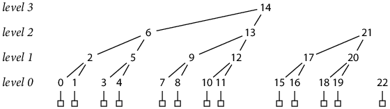
In the diagram, each hash is numbered and aligned horizontally according to its location in the interlaced file.
The postorder numbering makes the hash file append-only: each new record completes between 1 and lg N new hashes (on average 2), which are simply appended to the file, lower levels first.
Reading a specific hash from the file can still be done with a single read at a computable offset, but the calculation is no longer completely trivial. Hashes at level 0 are placed by adding in gaps for completed higher-level hashes, and a hash at any higher level immediately follows its right child hash:
seq(0, K) = K + K/2 + K/4 + K/8 + ...
seq(L, K) = seq(L–1, 2 K + 1) + 1 = seq(0, 2L (K+1) – 1) + L
The interlaced layout also improves locality of access.
Reading a proof typically means reading one hash
from each level,
all clustered around a particular leaf in the tree.
If each tree level is stored separately,
each hash is in a different file and there is no possibility of I/O overlap.
But when the tree is stored in interlaced form,
the accesses at the bottom levels will all be near each other,
making it possible to fetch many of the needed hashes
with a single disk read.
Appendix B: Inorder Storage Layout
A different way to interlace the lg N hash files would be to use an inorder tree numbering, in which each parent hash is stored between its left and right subtrees:
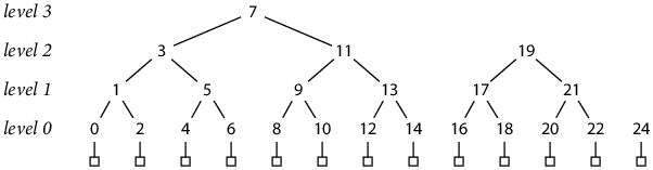
This storage order does not correspond to append-only writes to the file, but each hash entry is still write-once. For example, with 13 records written, as in the diagram, hashes have been stored at indexes 0–14, 16–22 and 24, but not yet at indexes 15 and 23, which will eventually hold h(4, 0) and h(3, 1). In effect, the space for a parent hash is reserved when its left subtree has been completed, but it can only be filled in later, once its right subtree has also been completed.
Although the file is no longer append-only, the inorder numbering has other useful properties. First, the offset math is simpler:
seq(0, K) = 2 K
seq(L, K) = 2L+1 K + 2L – 1
Second, locality is improved.
Now each parent hash sits exactly in the middle of its
child subtrees,
instead of on the far right side.
Appendix C: Tile Storage Layout
Storing the hash tree in lg N separate levels made converting to tile storage very simple: just don’t write (H–1)/H of the files. The simplest tile implementation is probably to use separate files, but it is worth examining what it would take to convert an interlaced hash storage file to tile storage. It’s not as straightforward as omitting a few files. It’s not enough to just omit the hashes at certain levels: we also want each tile to appear contiguously in the file. For example, for tiles of height 2, the first tile at tile level 1 stores hashes h(2, 0)–h(2, 3), but neither the postorder nor inorder interlacing would place those four hashes next to each other.
Instead, we must simply define that tiles are stored contiguously and then decide a linear tile layout order. For tiles of height 2, the tiles form a 4-ary tree, and in general, the tiles form a 2H-ary tree. We could use a postorder layout, as in Appendix A:
seq(0, K) = K + K/2H + K/22H + K/23H + ...
seq(L, K) = seq(L–1, 2H K + 2H – 1) + 1 = seq(0, 2H·L (K+1) – 1) + L
The postorder tile sequence places a parent tile immediately after its rightmost child tile, but the parent tile begins to be written after the leftmost child tile is completed. This means writing increasingly far ahead of the filled part of the hash file. For example, with tiles of height 2, the first hash of tile(2, 0) (postorder index 20) is written after filling tile(1, 0) (postorder index 4):
The hash file catches up—there are no tiles written after index 20 until the hash file fills in entirely behind it—but then jumps ahead again—finishing tile 20 triggers writing the first hash into tile 84. In general only the first 1/2H or so of the hash file is guaranteed to be densely packed. Most file systems efficiently support files with large holes, but not all do: we may want to use a different tile layout to avoid arbitrarily large holes.
Placing a parent tile immediately after its leftmost child’s completed subtree would eliminate all holes (other than incomplete tiles) and would seem to correspond to the inorder layout of Appendix B:
But while the tree structure is regular, the numbering is not. Instead, the offset math is more like the postorder traversal. A simpler but far less obvious alternative is to vary the exact placement of the parent tiles relative to the subtrees:
seq(L, K) = ((K + B – 2)/(B – 1))B || (1)BL
Here, (X)B means X written as a base-B number, || denotes concatenation of base-B numbers, (1)BL means the base-B digit 1 repeated L times, and the base is B = 2H.
This encoding generalizes the inorder binary-tree traversal (H = 1, B = 2), preserving its regular offset math at the cost of losing its regular tree structure. Since we only care about doing the math, not exactly what the tree looks like, this is probably a reasonable tradeoff. For more about this surprising ordering, see my blog post, “An Encoded Tree Traversal.”